Distance Analysis
Using a Cost Surface to Create an Optimal Path and Habitat Corridor
For this assignment I created a simplified cost surface and used it in distance analysis to create an optimal path and travel corridor between two different patches of deer habitat near the city of Fort St. John British Columbia.
Setting up the Analysis
The first step was to analyze all of the data given to me and set up my raster analysis environments in ArcGIS Pro.
Organizing the Data
To create a cost surface, I began by developing a chart to classify the surfaces that were preferred and disliked by deer. I selected three attributes, namely land cover, aspect, and slope, and then assigned weights to them based on data provided by a fictional biologist for this assignment. Subsequently, I established 10 preference classes (ranging from 1 to 10) and categorized each attribute based on the deer's preferences. For instance, since deer favor flat terrain over steep slopes, cells with no slope were allocated a preference rating of 1, while cells with steep slopes received a preference rating of 10.

Creating the Surfaces
As depicted in the Model, I generated three surface rasters, namely Land use, slope, and aspect. I accomplished this by utilizing a DEM raster as the input into two Surface Parameters tools and specifying slope and aspect as the parameters. The resulting outputs were a slope surface and an aspect surface, respectively.
Next, I utilized the Reclassify tool in conjunction with the provided aspect preference data to reclassify the aspect surface into an aspect preference surface. Additionally, I employed the slice tool to divide the range of slope into 10 categories, from least to most.
Regarding the land cover surface, I employed the Fort St. John land use land classification raster as the input surface into the Reclassify Tool and then used the provided ascii text file to help reclassify the different types of land cover into different preference categories. This output was a deer land cover preference surface.
Combining the Preference Surfaces
Finally I combined the three surfaces together using the Weighted Sum tool. The output of this was my weighted cost surface.

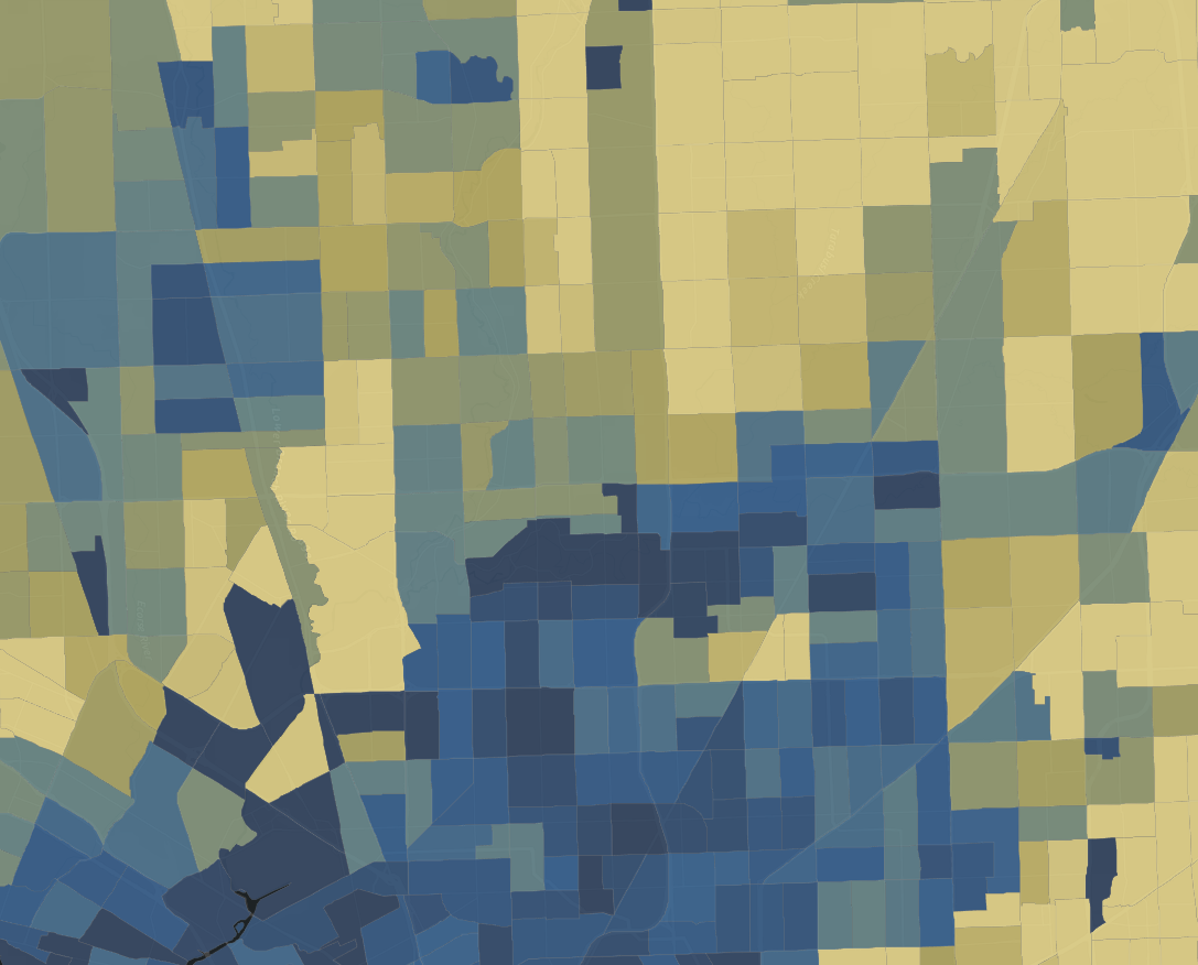
The final weighted cost surface which weighs each cell based on how much deer like the combination of slope, aspect and land use. Areas of the darkest red have a cost value of 37 and darkest green have a cost value of 4.
Using the Cost Surface in Distance Analysis
Create a Least-Cost Accumulation Surface Raster
This surface will show the accumulative “cost” for a deer to travel over the cost surface from any cell on the surface to a specific location. It will also create a distance back raster (Out Back) as any route to a location may have a different least cost route back.
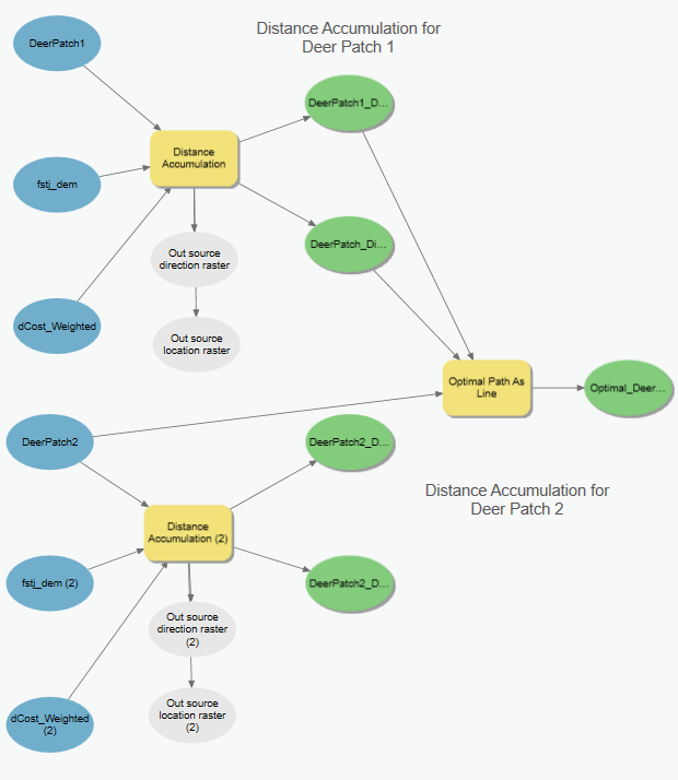
To accomplish this, I used the Distance Accumulation tool with Deer Patch as the source, the weighted cost surface as the input cost raster parameter and the Fort St John DEM as the surface raster (to calculate the surface-length of travel). The outputs were a distance accumulation raster and a distance back raster for each of the deer patches. This was a global operation.


Distance Accumulation Raster with legend showing that green indicates least cost travel through cells (aka areas of that deer have a high preference for) vs red areas that deer least prefer. I overlaid the roads layer for reference, you can note that this model does not take various roads into account.


The distance back raster shows the directions to follow from any single cell on the surface to get back to the source (The grey dot in the north east corner)
The final step in this model is to run the Optimal Path as Line tool that will calculate the best path from Deer Patch 2 to Deer Patch 1. This produces the single most efficient path of travel but as we know, deer tend to wander, so I used this raster as in input in the next step, creating an optimal corridor.
Creating an Optimal Corridor
Optimal Corridor Tool
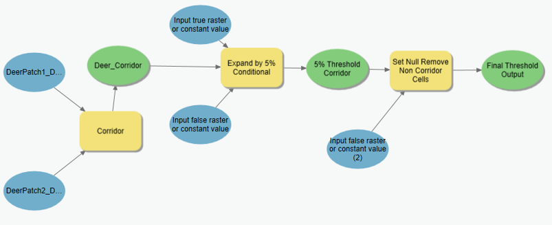
The corridor tool is similar to a buffer in that it is used to expand the optimal path that connects the two patches of deer habitat, but differs in that it takes into account the least cost path values. It takes the distance accumulation raster and the back direction raster and gives the sum of the accumulative cost to reach Deer Patch 1 from Deer Patch 2. I used the conditional tool to create a threshold value, the threshold meant that all cells with values less than the threshold would be included in this “buffer” and would represent cells that met my least cost travel requirements and therefore a swath of land that was most preferable to deer travel/habitat. (See image below)


Setting the Conditional Threshold
I ran the output of the corridor tool into a conditional tool and set the threshold for 10%. The initial result was too high so I adjusted the value to 5% and found the results with 5% covered an ideal amount of area (of course, in the real world, there would be much more consultation on choosing the threshold)
The conditional tool works as follows. If any cell values are equal or less than 149,427.6 (Which is the lowest least cost path value + 5% —> 142,312 + 7,115,5 = 149,427.6) assign a value of 1 to that cell. All other cells, assign a value of zero.
The resulting raster still displayed values of zero so I added another tool to set those values to null in order to only display the 5% threshold area.
The result of the Corridor tool (Deer Corridor) before implementing a threshold. The values are the sum of the cost of each cell travelling from Deer Patch 2 (yellow) to Deer Patch 1. (white). The blue line is the optimal path.

The 10% threshold deer corridor completely enveloping the city of Fort St. John.
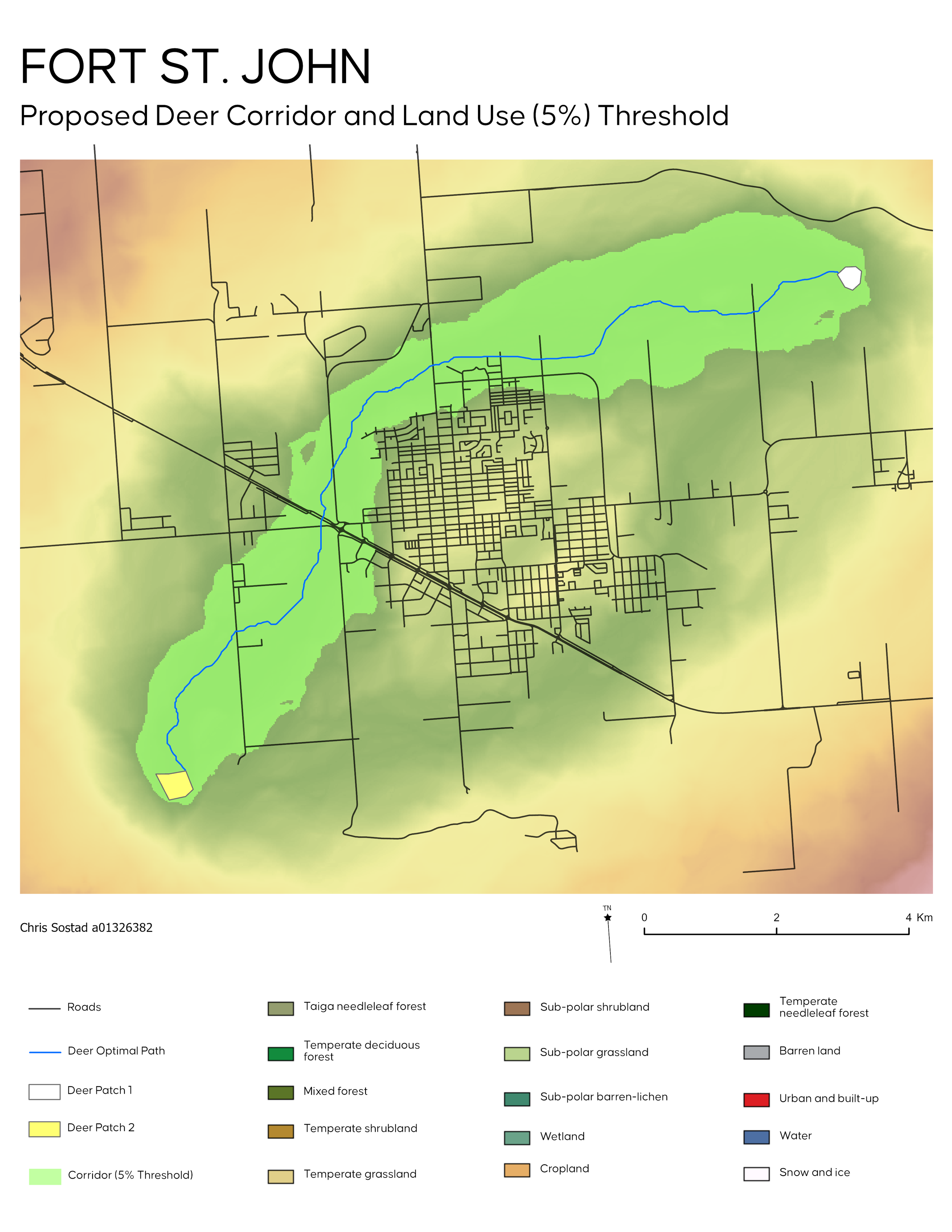
The Final Output - 5% Threshold
Conclusion
The final output could have be designed in many ways, I chose to display land Use in relation to the threshold. The overall model was simplified in many ways. As you can see from the map, there are many major roads running through my corridor and I didn’t take roads into account when calculating my cost rasters. This would be one area where the model could be improved. The weights I applied were relatively arbitrary and should have been analyzed by biologists. My chosen threshold was not based on any criteria, this was another area where more data would be required and further analysis done to choose an appropriate threshold.
Course material created by Carmen Heaver - BCIT